This Python library allows to apply a variety of different dimension reduction techniques on numpy and xarray objects. These include:
PCA (EOF analysis)
Maximum Covariance Analysis (MCA)
To simplify the interpretation of the results obtained from these xMCAalso offers regularization in the form of rotation:
Varimax-orthogonal rotation
Promax-oblique rotation
The new feature of xMCA, however, is the possibility to perform complex PCA and complex MCA, which are particularly suitable, when the covariance-describing patterns do not rest statically in space, but rather behave like a cyclic wave propagating in space.
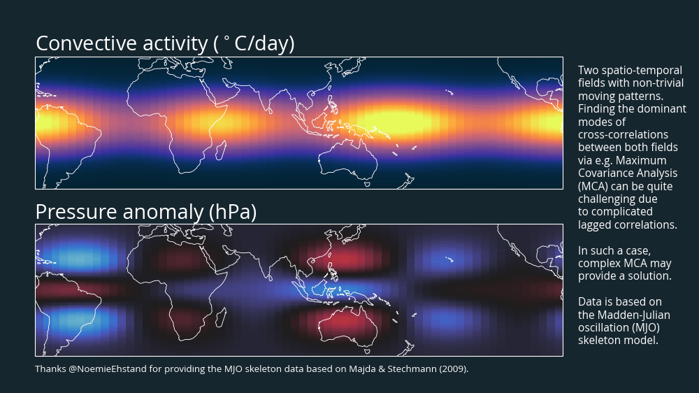
An example: the Madden-Julian oscillation
The Madden-Julian Oscillation (MJO) is just such a phenomenon. Made famous by the work of Madden and Julian (1971), it describes a system of very high and deep convective clouds occurring every 30 to 60 days and propagating eastward along the tropical Indian and Pacific Oceans. While there can be increased storm and rainfall activity within the convective zone, the eastern and western flanks of the system are mostly characterized by dry and sunny spells.
The following animation shows the convective activity as well as the sea level pressure anomaly, highlighting that the two variables are dynamically linked due to their common eastward motion. Due to the spatial waves, each point on the map affected by the signal experiences a phase shift, making it difficult for standard MCA to summarize the joint dynamics in a meaningful way.
This is where complex MCA comes in, which by design is perfect for capturing and compressing out-of-phase signals.
The benefits of using complex MCA
As the name suggests, in complex MCA the (complex) analytical signal is first formed for each (real) time series and then, analogous to standard MCA, the complex covariance matrix is decomposed by SVD. The obtained complex singular vectors (EOFs) and corresponding complex projections (PCs) together with the respective (real) singular values result in a set of modes, where the first mode describes the largest possible portion of phase-shifted covariance. This admittedly rather brief description may serve as a rough orientation for some, but if you want to know more details, please refer to the publication.
For a clear interpretation of the results of a complex MCA it is sufficient to understand that the complex EOFs/PCs also contain phase-shifted signals.
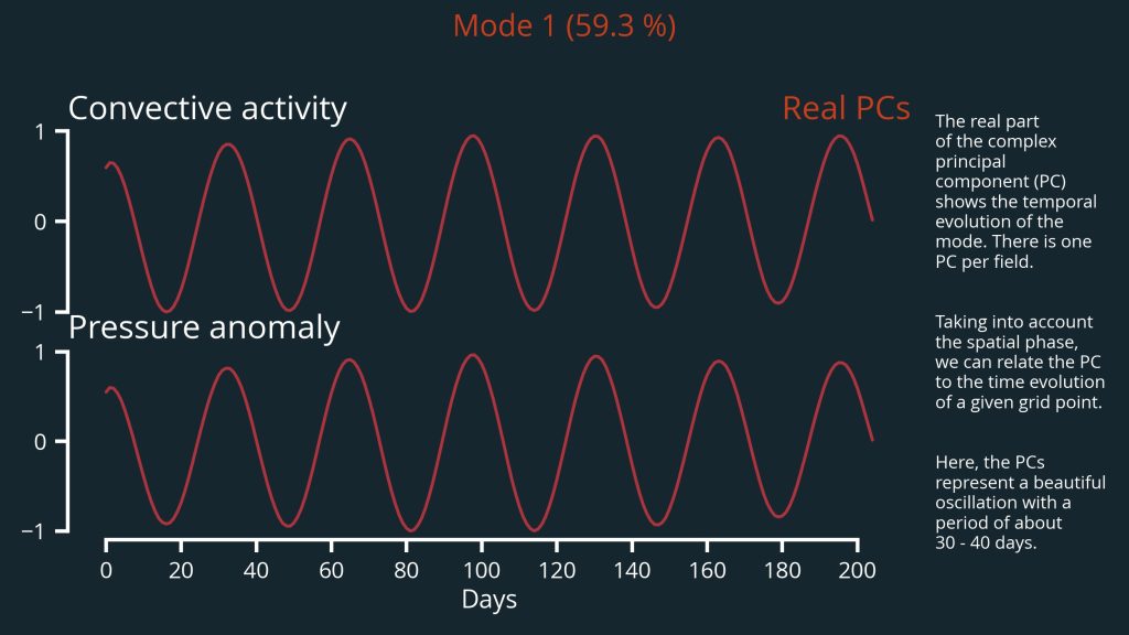
(Real) PCs of mode 1
In analogy to standard MCA the PCs reflect the temporal evolution of the given mode. In this case it is sufficient to look at the real part of the complex PCs (see figure below), because the imaginary part contains only a phase shift of 90º compared to the real part.
However, it is important to realize that unlike standard MCA, the real part provides only qualitative information about the time evolution of the mode. Thus, it would be wrong to conclude from the following graph that mode 1 is negative after about 80 days. This ultimately depends on the phase shift at a given location (more on this later).
The complex PCs are thus defined only up to the phase shift, that is, each phase-shifted pair of PCs is in turn a valid PC pair. The phase-shifted PCs are also consistent with the corresponding EOF pair as long as the phase shift is applied to the EOFs as well.
The real PCs of both fields of mode 1 are characterized by an oscillation with an approximate period of 40 days. This mode describes about 60% of the (phase-shifted) covariance present in the data.
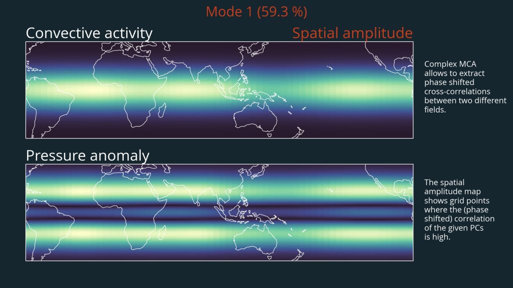
Spatial amplitude
In analogy to the EOFs of standard MCA, the spatial amplitude As provides a means to understand which regions contribute the most to the given mode. The spatial amplitude is easily computed via the complex EOF and the complex conjugate EOF*
From the following figure it is clear that the oscillation of convective activity is mainly dominant around the equator, while most of the oscillations of pressure anomalies occur in the extra-tropics and to a lesser extent over the ITCZ.
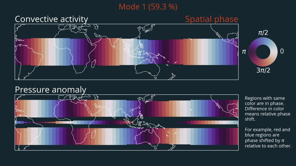
Spatial phase
Now this is the really interesting part. Using the spatial phase,
we can determine exactly how the individual regions are dynamically linked to each other. Regions with the same color are in phase, i.e. their time series correlate with each other, while regions whose color is πapart are anti-correlated. Phase shifts between these two cases are signals that could not be combined into one mode with standard MCA.
As mentioned above, the time evolution of the respective mode can be calculated on the basis of the complex PC and the respective phase shift at a certain location.
Based on the fact that there are 3 regions in phase along the equator at the same time, the wavenumber 3 of this MJO mode can be inferred.
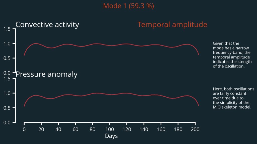
Temporal amplitude
Now, the temporal similarly defined as
is easy to understand. It just gives an estimate of the strength of the mode at a given moment in time, and as such is the analog of the PCs when using standard MCA. In principle, it could be directly compared to traditional measures like the MJO amplitude provided by Wheeler and Hendon (2004)
Due to the simplicity of the MJO skeleton model which was used to create the example data sets, the amplitude rests fairly constant. In the real world, this would look very different.
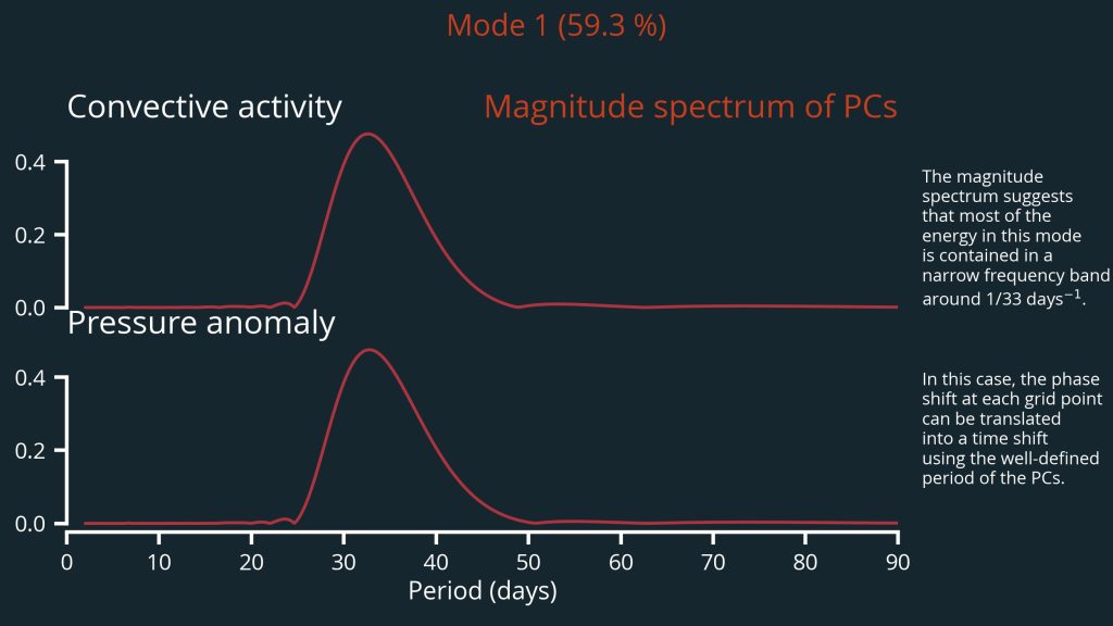
Magnitude spectrum of PCs
The analysis of the magnitude spectrum of the PCs is an integral part of the complex MCA. Because only if the energy of the mode is concentrated in a relatively narrow frequency range, the phase can be easily converted into a time shift. If this is given, then in principle not only phase-shifted but also time-shifted signals can be determined.
In this sense, complex MCA is particularly suitable in cases where solar, seasonal, or lunar cycles are to be studied. Unfortunately, this is not always the case and many processes in the climate system are in fact a mixture of very different frequencies.
Nevertheless, complex MCA does not hurt. Even in the case of very broadband modes, in-phase (correlated) and out-of-phase (anti-correlated) signals can always be interpreted in terms of a standard MCA.
Acknowledgments
MJO data: Thanks to Noémie who provided me with the simulation data for the MJO skeleton model within a very short time thanks to her excellent Julia skills.
Colormaps: The colormaps used here are all from cmocean. Kudos to the developer for making their extremely aesthetic taste available to the masses.
Funding: This work is part of the Climate Advanced Forecasting of Sub-Seasonal Extremes (CAFE) project. We gratefully acknowledge funding from the European Union’s Horizon 2020 research and innovation programme under the Marie Skłodowska-Curie Grant Agreement 813844.