IT ADM – Page 2

The Rossby Wave Packets

Posted on March 11, 2022March 11, 2022 by IT ADM

The Rossby Wave Packets

Iago Pérez | Universidad de la República, Montevideo

___________________________________________________________________________________________

Importance of the Rossby Wave Packets in the Atmosphere

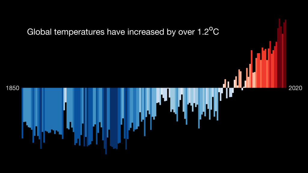
We all have experienced (or will experience) the intensity of an extreme meteorological weather event in our lives, for example, persistent high temperatures during a heatwave or intense rainfall due to the development of an extratropical cyclone. Even if these events do not appear very often, they cause severe human and economic losses in the areas they cross. For example, the European heatwave of 2003 caused around 30.000 deaths in Europe and a water shortage that severely affected food production and even caused the shutdown of nuclear power facilities in France. In addition, several studies have shown that these extreme weather events will appear more often and with higher intensities due to the climate change induced by human activity.

Therefore, it is key to improve the detection of extreme weather events with sufficient advance to apply mitigation measures and lessen future damages. Nonetheless, before forecasting the apparition of extreme weather events, we need to understand what physical mechanisms trigger their development in the first place. One of the processes that can trigger the development of extreme weather events is the propagation of Rossby Wave Packets.

What are Rossby Wave Packets?

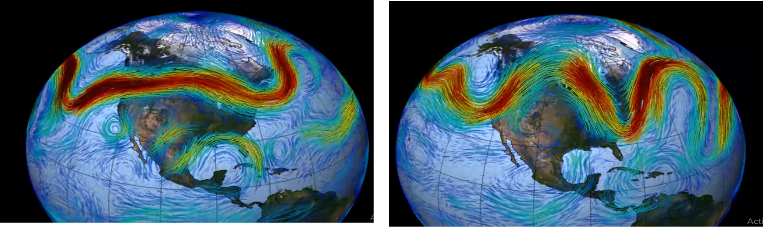
What exactly are Rossby Wave packets? They are meanders, deviations of the strong westerly winds that travel at the high atmosphere of mid-latitudes from west to east that travel by what is called “downstream development mechanisms”. Normally, the strong westerly winds travel around the Earth forming a belt-like pattern but when a Rossby Wave Packet appears, the wind flow shows strong oscillations that resemble a snake movement (Figure 1). These “atmospheric snakes” are the Rossby Wave packets traveling in the atmosphere, and during their lifetime they transport huge quantities of energy modifying the weather in the areas they cross. Intense and narrow currents of westerly winds act as a highway for the RWPs and are where they gain enough stability to last longer periods in the atmosphere, under certain circumstances, from several days to 2-3 weeks before disappearing. These packets, due to all the energy they carry, are considered precursors of extreme weather events, and also increase the complexity and uncertainty of the meteorological forecast in the areas they cross. These phenomena appear in both the northern and southern hemispheres.

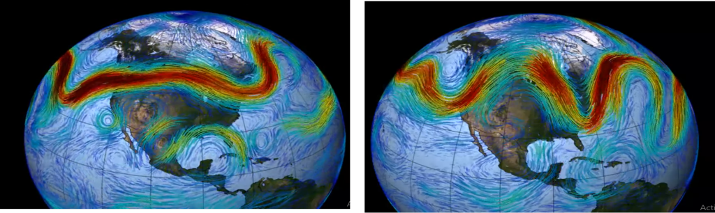
Figure 1: representation of the usual flow of the jet stream in the Northern Hemisphere (left) and during the propagation of a Rossby Wave Packets(right) , greenish and reddish areas indicate the main wind flow course. (https://https://oceanservice.noaa.gov/facts/rossby-wave.html)

If we can understand which processes favor the development of these long-lived packets, we would be close to knowing what phenomena can shape weather and climate in the mid-latitudes and enhance the detection of extreme weather events between 10-30 days. Thus, my research focuses on the study of the climatological conditions which favor the apparition of Rossby Wave Packets that last more than 8 days in the atmosphere, (which are wave packets with great stability and energy), and to identify under which circumstances the meteorological forecast can correctly predict the apparition of these long-lived packets in the Southern hemisphere.

State of the art of the study of Rossby Wave Packets and the importance of climate modes in the Southern Hemisphere climate.

Until not long ago, the study focused mainly on the Northern Hemisphere whereas on the Southern Hemisphere there were fewer studies, and they did not focus on the influence of climatological events in the frequency of occurrence of these packets. It is important to fill this gap of information in the Southern Hemisphere to have a more complete understanding of how the Earth climate system works to increase the reliability of the meteorological forecast systems.

In one of our research studies, we observed how long-oscillating trends of the weather affect the formation and propagation of long-lived Rossby Wave Packets during Southern Hemisphere summer (December to March). The climatic trends studied in that research are:

1.-El Niño Southern Oscillation, (ENOS): it is one of the most important and studied climate modes. It consists of a changing pattern of sea surface temperature in the tropical Pacific that triggers the development of processes that modify the weather on a global scale. When the tropical Pacific sea surface temperature is warmer (cooler) than the average, is signaling the manifestation of El Niño (La Niña) event (Figure 2).

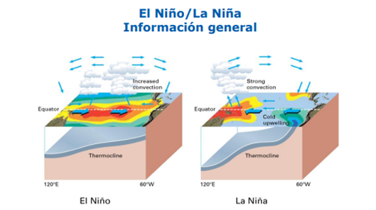
Figure 2: Wind circulation flow and oceanic circulation anomalies caused in the tropical Pacific during El Niño events (left) and La Niña (right). During El Niño years, we have sea surface temperature above average in the Tropical Pacific due to the inversion of the usual wind circulation, introducing hot surface water in the eastern Pacific basin. On the other hand, during La Niña events, the usual wind flow is strengthened, bringing to the surface cold sub-superficial water that cools the sea surface temperature.

2.-Southern Annular Mode, (SAM): it consists of the displacement of strong westerly winds between high and mid-latitudes in the Southern Hemisphere due to the changes in superficial pressure located in the center of the Antarctic. It has two stages, SAM – and SAM +. In SAM + stages, the pressure at the Antarctic is below the usual, causing the apparition of a low-pressure cell that causes the displacement of strong westerly winds towards high latitudes. As a result, the cold and humid winds are contained far away from the Southern American continent and enable the development of sunny weather and high temperatures. On the other hand, during SAM – we have the opposite effect, this is, the pressure in the center of the Antarctic is above the usual, so the strong westerly winds now move towards subtropical latitudes, bringing rainfall and cold and humid winds to South America (Figure 3).

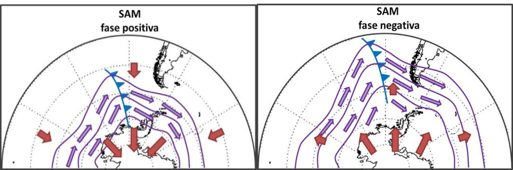
Figure 3: Stages of Southern Annular Mode or SAM. Red arrows go from the highest areas of pressure to the lowest,
purple shows the resultant main wind circulation and blue lines show the development of a cold front.
Source: http://met-ba.blogspot.com/2015/09/30-9-2015-oscilacion-antartica-o-modo.htm

Latest findings

We observed how ENSO and SAM, affect the propagation of long-lived RWPs during the austral summer (December- March) of the Southern Hemisphere from 1979 to 2020. The results obtained in this study suggest that during years of negative SAM, we will observe more extreme weather events caused by the apparition of these long-lived packets. Thus, extreme weather event detection in the meteorological forecast between 10-30 days in advance should be more precise during negative SAM years, and less accurate during years with La Niña/positive SAM events because these wave packets should be more easily represented during years in which the atmospheric conditions favor their apparition.

During years with SAM – events, there are more long-lived Rossby Wave Packets compared to its opposite stage, (SAM +), and these packets last significantly longer in the atmosphere. Because these wave packets need a strong and narrow westerly wind to propagate, we concluded that these differences are due to the two motives:

1st During negative SAM years, the strong westerly winds are generally more intense and show a narrower distribution in the mid-latitudes compared to the wind regime during SAM + years, acting as a better highway where RWPs can last longer in the atmosphere.

2nd An anticyclone cell is developed in the Southeast of Australia during years of SAM +, blocking the jet and the propagation of Rossby Wave packets, whereas in years of SAM – this blockage is either absent or more confined in more tropical latitudes (Figure 4).

Therefore, the atmospheric conditions established in years with SAM – support the development of more stable RWPs that last longer in the atmosphere compared to its opposite stage.

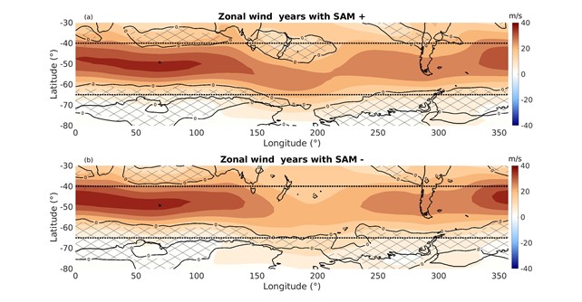
Figure 4: Mean wind flow during years with SAM + (up) and SAM – (down) events. Colored areas show the intensity of the wind speed in the eastward direction. Gridded areas highlight locations where the wind flow impedes or damps the propagation of Rossby Wave Packets.

In the case of ENSO, we found that during El Niño events we detected more long-lived RWPs compared to La Niña. Nonetheless, this tendency is as not as robust as in the previous pattern, and the changes in the wind flow are not as obvious as those during different SAM stages. Therefore, we assumed that this relationship is found because El Niño contributes to the development of atmospheric conditions that favor the manifestation of SAM –, and La Niña does the same with SAM +. Nonetheless, it is important to highlight that the presence of El Niño or La Niña event is not the only factor that determines the main stage of SAM. This may explain why this connection is not as strong as the previous pattern.

Now, in our next project we are trying to measure the extent to which the actual meteorological models can correctly predict the apparition of these long-lived RWPs, and how similar are the predicted packets against the original trajectories. In other words, if the predicted trajectory of the long-lived RWPs appears in the same area as the real RWPs or if the predicted packets last the same as the originals etc. If you want to know more about it, stay tuned!

Further Reading

Original publication: https://agupubs.onlinelibrary.wiley.com/doi/10.1029/2021JD035467

Climate change and its influence in future climate https://www.ipcc.ch/2021/08/09/ar6-wg1-20210809-pr/

Definition of Southern Annular Mode or SAM: http://www.bom.gov.au/climate/sam/

Information about the Nez Zealand blockage: Hendon, H., & Hendon, H. H. (2018). Understanding Rossby wave trains forced by the Indian Ocean dipole. Climate Dynamics, 50(50), 2783–2798. https://doi.org/10.1007/s00382-017-3771-1

Effect of ENSO in SAM: https://doi.org/10.1175/2010JAS3311.1

Impact of the 2003 heatwave: https://www.britannica.com/event/European-heat-wave-of-2003

Entrevista de Predictia a Riccardo Silini, doctorando de CAFE

Posted on February 22, 2022February 22, 2022 by IT ADM

Entrevista de Predictia a Riccardo Silini

Riccardo Silini| Universitat Politècnica de Catalunya, Barcelona

___________________________________________________________________________________________

Hablamos con: Riccardo Silini, doctorando de CAFE

Viernes 11 de febrero 2022

Los eventos climáticos extremos dejan tremendos impactos en la sociedad. Solo en 2021, tal y como detalla la Organización Meteorológica Mundial en su ‘Estado del Clima de 2021’, los impactos de los eventos climáticos han sido enormes. La temperatura hizo que lloviese por primera vez – en vez de nevar – en el hielo de Groenlandia. Los glaciares canadienses sufrieron un rápido deshielo. Canadá y las zonas cercanas de EE. UU. sufrieron una ola de calor en las que se llegó a casi 50ºC. El valle de la muerte de California registró 54.4 ºC como pico en una ola de calor y muchas partes del mediterráneo tuvieron temperaturas récord. En China, la cantidad de lluvia que habitualmente cae en varios meses, cayó en apenas unas horas y diversas partes de Europa se inundaron, causando docenas de muertes y daños millonarios. En Sudamérica, la reducción en el caudal de los ríos impactó la agricultura, el transporte y la producción de energía de numerosos países.

Por eso, investigar y comprender cómo se producen estos fenómenos extremos es de vital importancia. Nos permite estar más preparados, predecirlos con mayor precisión y en definitiva tener más control sobre su impacto. Una de las iniciativas de las que formamos parte busca investigar sobre eventos climáticos extremos, para así mejorar nuestra comprensión sobre ellos. Se trata de CAFE, una ITN: una red que une a investigadores, industria y conocimientos especializados en climatología, meteorología, estadística y física no lineal. El objetivo es entrenar a diversos diversos doctorados, cuyas tesis están relacionadas con el clima extremo. En total, 20 instituciones entre beneficiarios y socios, lideradas por el Centre de Recerca Matemática. Dentro de esta red, desde Predictia funcionamos como “hogar de acogida” durante un periodo de tiempo para algunos de los doctorandos de la red, y así complementar su formación y que puedan ejecutar proyectos concretos.

Hoy entrevistamos a uno de estos doctorandos, Riccardo Silini, a punto de defender su tesis. Su investigación gira en torno a dos temas: el primero es un fenómeno climático muy específico, conocido como la oscilación Madden-Julian (los detalles, más adelante), y un método estadístico para analizar la causalidad entre diferentes fenómenos. Para hablar de todo ello, quién mejor que el propio Riccardo.

Antes de meternos en harina, cuéntanos un poco sobre ti.

Vengo de Suiza, donde obtuve me licencié e hice un máster en Física en física en la EPFL. Me centré principalmente en las redes complejas, las neurociencias teóricas y la inteligencia artificial. Actualmente estoy haciendo mi doctorado en el proyecto ITN CAFE en la UPC en Barcelona, que gira en torno a la previsión de los extremos climáticos sub-estacionales.

Una parte de tu investigación gira en torno a la oscilación Madden-Julian. ¿Cómo explicarías este fenómeno para alguien que se encuentra este término por primera vez?

Se trata de un fenómeno que afecta a una zona muy concreta del mundo: desde el oeste de África hasta el océano Pacífico. Es un patrón atmosférico cuyo efecto directo es dejar precipitaciones anómalas y su característica principal es que tiene dos zonas: una con más precipitaciones de lo habitual y otra con menos.

La oscilación de Madden-Julian deja dos zonas diferenciadas, una más lluviosa y otra más seca, que se desplaza hacía el este | Fuente: cazatormentas.net

Además de las propias lluvias que genera la oscilación, ¿por qué es importante predecir su comportamiento?

Además de dejar más o menos precipitaciones, influye en los monzones de verano del oeste de África y de la India. Y yendo más allá, tiene una conexión bidireccional con El Niño (El Niño es influido por la MJO y al revés).

Lo que hace que está oscilación de Madden-Julian sea más complicada de predecir es que a veces está activa y a veces inactiva, como si tuviera un interruptor. Para indicarnos si la MJO está activa o no, miramos un índice, llamado RMM, que sirve para indicarnos si este fenómeno está activo o no. Mi tesis consiste en mejorar la predicción de este índice, utilizando un enfoque de Machine Learning.

¿Podrías contarnos un poco más de detalle?

Para aquellas personas que quieran meterse en detalles técnicos, hay un paper que hemos publicado en npj Climate and Atmospheric Science. En este paper aplicamos dos enfoques para la predicción. El primer enfoque es de Machine Learning puro: empleo un tipo concreto de redes neuronales, intentando mantener unas redes neuronales lo más simple posible. Como es de esperar, el desempeño de estas redes por sí solas no supera al de los modelos climáticos. Esto es normal, porque los modelos climáticos llevan detrás toda la física de la atmósfera, y por tanto simulan la realidad. Sin embargo, este enfoque de Machine Learning sí que supera a otros métodos más simples. Además, comparado con los modelos climáticos, que son computacionalmente muy pesados, el enfoque de Machine Learning es mucho más ligero.

Este primer enfoque encaja muy bien en una de las eternas discusiones que vemos en el ámbito de la Inteligencia Artificial: la rivalidad amistosa entre la gente que opina que es mejor utilizar modelos numéricos y los que opinan que es mejor aplicar Machine Learning, Deep Learning u otras técnicas. ¿En qué parte de este espectro te situarías?

Como todo, depende de la aplicación concreta. En mi caso, para las simulaciones de clima y meteo… creo que es mejor tirar por la calle de enmedio y dejar que cada técnica aporte su mejor parte. Me explico: los modelos numéricos simulan muy bien la física que hay detrás de fenómenos atmosféricos, y nos dan una información muy valiosa. Por tanto, tiene sentido que usemos estos modelos como una primera aproximación, en vez de gastar tiempo y recursos en que una red neuronal “aprenda de cero” estos fenómenos. No tiene sentido poner este peso de aprendizaje en la red cuando ya conocemos esa física.

Este es justo el segundo enfoque que exploramos en el paper. Tomamos de partida un modelo numérico, e intentamos mejorar sus predicciones, post procesando con Machine Learning. En concreto utilizamos el mejor modelo numérico que hay actualmente, desarrollado por el ECMWF, que tiene la mejor skill de predicción para la oscilación de Madden-Julian. Entonces tomamos una red neuronal (feed-forward neural network) y la entrenamos para que corrija los resultados del modelo. El resultado es un post proceso que mejora la predicción del modelo numérico y que también es mejor que otros tipos de postprocesado más clásicos, como una regresión lineal múltiple.

Otro aspecto interesante es que hemos visto que también mejora un aspecto muy concreto de la predicción: cuando la oscilación de Madden-Julian está a punto de entrar en el continente marítimo, la física se vuelve más compleja, y la habilidad de predicción de los modelos numéricos cae. Es justo en este punto en el que la corrección con Machine Learning tiene el mayor efecto, porque llega a corregir bastante bien esta caída del skill.

En resumen, creo que lo más útil es dedicar recursos a mejorar las dos cosas: mejorar los modelos numéricos a medida que vamos descubriendo nuevos aspectos de la física que hay detrás; y mejorar el post proceso de Machine Learning, que cubren esa última distancia entre modelos y realidad, para hacer predicciones más precisas.

Vamos a cambiar de tema, para hablar de otro de los focos de interés de tus investigaciones: la causalidad. ¿Nos puedes explicar un poco de dónde parte tu interés?

En nuestro día a día, normalmente no tenemos problema en ver la causalidad directamente. Si pegamos una patada a una pelota, sale disparada. Sin embargo, cuando nos movemos en ámbitos más abstractos o complejos… la causalidad cuesta un poco más de ver.
El ejemplo perfecto lo tenemos en el tiempo atmosférico: son sistemas complejos, con multitud de partes individuales que interaccionan entre sí y tienen efectos que no podríamos saber estudiando cada parte por separado.

Ilustración de la causalidad de Granger | Fuente: BiObserver, CC BY-SA 3.0, via Wikimedia Commons

Sin embargo, se puede usar la idea de causalidad en cualquier ámbito, no sólo clima.

Exacto. En mi caso, partimos de muchas series temporales que nos dicen cómo evolucionan varios parámetros de forma separada. Con esa cantidad de información, es difícil ver las relaciones que unas cosas guardan con otras.

En estadística, uno de los métodos que usamos para ver esta causalidad es la causalidad de Granger. Más que decir si X causa Y, nos indica si X predice Y. La causalidad de Granger nos da una métrica, un indicador, de cómo de bueno es un parámetro para predecir el comportamiento de otro parámetro.

Y justo lo que estás investigando es un método para mejorar estas métricas.

Sí. Hemos desarrollado una herramientaque permite hacer un análisis de la causalidad, entendida en el sentido de Granger que mencionaba anteriormente: más que decir que X causa Y, nos permite decir que X predice Y. Los detalles tećnicos están en este paper en scientific reports y el código para implementar el sistema está disponible en mi GitHub.

¿Cómo recomendarías usar esta herramienta?

Lo primero es que funciona con series temporales cortas, de 500 puntos. Esto es porque en ese tamaño, la librería es mucho más rápida que la librería de causalidad de Granger que ya existe en Python.

Lo segundo, es que se trata de una herramienta de diagnóstico rápido. En vez de analizar todas las opciones a fondo, nos permite hacer un estudio rápido de la información que tenemos para ver posibles relaciones de causalidad. La idea detrás de la librería es que el usuario dé como input una matriz con las series temporales a analizar y que obtengas como resultado una matriz de causalidad.

Lo que hemos visto es que aplicar esta métrica a diferentes problemas nos da buenos resultados. El ejemplo que comentamos en el paper está relacionado con índices climáticos. Lo que vemos es que reproduce muy bien las relaciones que ya conocemos entre diferentes índices. Entonces, como reproduce bien el conocimiento que ya sabemos, nos permite saber que hace un trabajo robusto… y nos permite explorar aquello que no sabemos. Si vemos dos índices climáticos que en la matriz de causalidad salen como relacionados, ya tenemos un camino por el que tirar: investigar más a fondo si eso es un falso positivo, o es posible que haya una relación de causalidad entre ellos.

La rapidez de la herramienta nos permite hacer un análisis amplio muy rápido. Además una de las características que hemos integrado en el código es bastante única: ver el impacto de una serie temporal con un lag. Esto es algo que no he podido encontrar en las librerías que existen actualmente, al menos en mi experiencia.

Y ahora que vas a estar una temporada en Predictia, ¿en qué estás cacharreando?

De momento no se puede contar mucho detalle, pero tiene que ver con índices de riesgo de fuego y causalidad.

Para saber más, habrá que esperar a que Riccardo termine su estancia con nosotros. ¡Permaneced atentos!

Enlaces interesantes:

La entrevista original de Predictia

Página web de Predictia

CAFE Researchers among the World's Top 2% in Academic Citation

Posted on February 18, 2022 by IT ADM

A total of nine researchers from the CAFE project appear on the updated version for the 2021 list and the career-long list, based on standardized information on citation metrics and other factors that measure the impact of a researcher’s work.

From top to bottom, left to right: Cristina Masoller, from Universitat Politècnica de Catalunya (UPC), Hervé Douville, from Météo-France, Pascal Yiou, from the Commissariat à l’énergie atomique et aux énergies alternatives, Jörg Matschullat, from the Technische Universitaet Bergakademie in Freiberg, Florian Pappenberger, from the European Centre for Medium-Range Weather Forecasts (ECMWF), Álvaro Corral, from the Centre de Recerca Matemàtica (CRM), Jürgen Kurths, from the Potsdam Institut fuer Klimafolgenforschung, Holger Kantz, from the Max Planck Institute for the Physics of Complex Systems, and Reik Donner, from the Potsdam Institut fuer Klimafolgenforschung

The Stanford University (USA) has recently released an update of the list that ranks the top two percent of the world’s most-cited scientists during 2020, including 9 team members from the CAFE project consortium, and the top two percent of the world’s most-cited scientists for career-long citations.

The prestigious single-year impact list includes Cristina Masoller, from Universitat Politècnica de Catalunya (UPC), Álvaro Corral, from the Centre de Recerca Matemàtica (CRM), Florian Pappenberger, from the European Centre for Medium-Range Weather Forecasts (ECMWF), Pascal Yiou, from the Commissariat à l’énergie atomique et aux énergies alternatives, Jörg Matschullat, from the Technische Universitaet Bergakademie in Freiberg, Hervé Douville, from Météo-France, Holger Kantz, from the Max Planck Institute for the Physics of Complex Systems, Jürgen Kurths, from the Potsdam Institut fuer Klimafolgenforschung and Reik Donner, from the Potsdam Institut fuer Klimafolgenforschung

About the study

The list, created by Professor John P. A. Ioannidis (an expert in data science) from Stanford University and his research team, contains a publicly available database that provides standardized information on citations, h-index, co-authorship-adjusted hm-index, citations to papers in different authorship positions, and a composite indicator. It is based on the bibliometric data included in the Scopus database, and comprises more than 100,000 researchers from 144 countries, out of 8 million scientists considered to be active worldwide (according to UNESCO data), classified in 22 scientific fields and 176 subfields.

Additionally, the study also includes a similar list compiling data for researcher’s entire careers, considering articles published between 1960 and 2019.

Original reference:

Baas, Jeroen; Boyack, Kevin; Ioannidis, John P.A. (2021), “August 2021 data-update for “Updated science-wide author databases of standardized citation indicators“”, Mendeley Data, V3, doi: 10.17632/btchxktzyw.3

CAFE Researchers among the World’s Top 2% in Academic Citation

Posted on February 18, 2022February 18, 2022 by IT ADM

A total of nine researchers from the CAFE project appear on the updated version for the 2021 list elaborated by experts from the University of Stanford, based on standardized information on citation metrics and other factors that measure the impact of a researcher’s work.

From top to bottom, left to right: Cristina Masoller, from Universitat Politècnica de Catalunya (UPC), Hervé Douville, from Météo-France, Pascal Yiou, from the Commissariat à l'énergie atomique et aux énergies alternatives, Jörg Matschullat, from the Technische Universitaet Bergakademie in Freiberg, Florian Pappenberger, from the European Centre for Medium-Range Weather Forecasts (ECMWF), Álvaro Corral, from the Centre de Recerca Matemàtica (CRM), Jürgen Kurths, from the Potsdam Institut fuer Klimafolgenforschung, Holger Kantz, from the Max Planck Institute for the Physics of Complex Systems, and Reik Donner, from the Potsdam Institut fuer Klimafolgenforschung

About the study

Additionally, the study also includes a similar list compiling data for researcher’s entire careers, considering articles published between 1960 and 2019.

Original reference:

Changing atmospheric circulations in a warming climate

Posted on February 3, 2022February 3, 2022 by IT ADM

Changing atmospheric circulations in a warming climate

Pedro Herrera Lormendez | Technische Universitaet Bergakademie Freiberg

___________________________________________________________________________________________

In recent decades, we humans have strongly influenced the behaviour of climate given the enormous amounts of “heat-trapping” gasses that we have emitted since the beginning of the industrial revolution. These greenhouse gasses have generated an increase in the Earth’s temperature and this has had an implication for the climate as we once knew it. More extreme meteorological events have become more common and they are expected to continue to affect us more strongly in the future. Events like longer-lasting heatwaves, droughts or intense flooding taking place where they were not common in the past will become the “new normal” of our daily news. But, why are these extreme events increasing and what causes them in the first place?

Atmospheric circulation patterns primarily determine the day-to-day weather we experience in our cities and regions, but what do you know about them? You usually see them displayed on the news during weather reports: High and low-pressure systems, warm and cold fronts as well as air masses are some of the most common words you might have heard. Anticyclones (pressure highs) and cyclones (pressure lows) are the two patterns that dominate the atmosphere. Many of the effects on the weather will depend upon the position, movement and intensity of these formations. While cyclones are mostly responsible for the rainy days we experience, they can also cause windy and snowy days during winter. They are also behind the formation of hurricanes in the tropical regions of the planet. Anticyclones, on the other hand, have the ability to inhibit precipitation and favour very cold periods during winter or heatwaves and droughts during summer.

Global temperature change since year 1850 (Ed Hawkins, https://showyourstripes.info/s/globe)

These atmospheric patterns have direct implications on the European climate and variables like temperature are strongly modulated by the occurrence of these circulations. Besides the main cyclones and anticylones mentioned above, we can also classify these atmospheric configurations depending on their dominant wind flow, which therefore relate to their influence on the dominant air masses that move over Europe. During winter (months of December, January and February, DJF) for example, two circulations overrule the contrast in temperatures that we experience. In principle, the constant flow of wind from the west (W) brings humid air from the Atlantic and promotes milder temperatures for most of the western part of the continent. However, the inverse occurs when the rarer events of (only 2.4% frequent) easterly winds (E) take place. They usually blow very cold and dry air masses from the continental part of Europe and Russia which give way to some of the coldest days that we endure during this season.

Influence of atmospheric circulations on winter (DJF) and summer (JJA) European temperatures (Herrera-Lormendez et al., 2021)

Unfortunately, these habitual climatic conditions that we are familiar with will likely bear significant changes in the coming decades given the progressive warming of the planet. Our current understanding of climatic science indicates that the tropical conditions that we usually observe below the 30º of latitude will tend to become the “new normal” for regions located further north (further south in the southern hemisphere). This means that given a general change in the global circulation we will also expect this to affect what happens in the smaller scale circulations. As an example, there is a high confidence that, by the end of the century, Northern Europe will experience more rainfall than usual during its winters. On the other hand, a significat reduction in precipitations future summers in the Mediterranean and Western Europe is expected.

Projected seasonal precipitation changes by the end of the 21st century (IPCC, 2021)).

Before we mentioned the increase of ‘heat trapping’ gasses, but what exactly is driving all these changes? To better grasp it, we evaluated past and predicted future variations in the dominant European atmospheric circulations from the 1900s to the 2100s. The future was assessed by using physical and mathematical numerical climate models that try to reproduce the behaviour of the climatic system under different possible scenarios. We assumed a worst-case scenario where we continue emitting greenhouse gasses without consideration. In this case, the results indicated that in winters, this projected increase in precipitation might relate to an escalation in the frequency of days characterised by westerly wind flow that brings humid air masses from the North Atlantic Ocean. In the summer, on the other hand, we would have more circulation changes. These suggest an increment in the easterly-wind dominated days (linked with warmer and drier summer days), whereas the frequency of milder and wetter westerlies will be coerced due to the increase of the first. We find that these long-term modifications to the climate as we know it will be inevitable by the mid 21st century if no actions are taken to reduce the emission of heat-trapping gasses.

Past and future changes in synoptic circulations over Europe (a to d) and probable times of emergence of these changes (e and f) (Herrera-Lormendez et al., 2021)

Nevertheless, it remains hard to quantify the exact time when these transitions will emerge and how exactly they will affect the regional aspects of our weather and climate as these depend on much more complex interactions between other components like vegetation coverage, urban growth, soil humidity, among others.

However, two things are clear:

First of all, we need more interdisciplinary studies in the matter to assess all the variables and interactions involved in the future impacts of climate change in the whole climatic system. Secondly, we need to take action now to try not to reach a situation anywhere close to the predicted “worst-case scenario” in our research. This would lead to a world and a society facing very difficult living conditions and fighting for the already under strained resources.

A more comprehensive and detailed discussion of this topic can be found in our recently published work in the International Journal of Climatology:

Herrera-Lormendez P, Mastrantonas N, Douville H, Hoy A, Matschullat J. 2021. Synoptic circulation changes over Central Europe from 1900 to 2100 – Reanalyses and CMIP6. International Journal of Climatology. John Wiley & Sons, Ltd. https://doi.org/10.1002/joc.7481

xMCA: A Python library for complex Maximum Covariance Analysis in Xarray

Posted on January 11, 2022January 11, 2022 by IT ADM

xMCA: A Python library for complex Maximum Covariance Analysis in Xarray

Niclas Rieger | Centre de Recerca Matemàtica

___________________________________________________________________________________________

This Python library allows to apply a variety of different dimension reduction techniques on numpy and xarray objects. These include:

PCA (EOF analysis)
Maximum Covariance Analysis (MCA)

To simplify the interpretation of the results obtained from these xMCA also offers regularization in the form of rotation:

Varimax-orthogonal rotation
Promax-oblique rotation

The new feature of xMCA, however, is the possibility to perform complex PCA and complex MCA, which are particularly suitable, when the covariance-describing patterns do not rest statically in space, but rather behave like a cyclic wave propagating in space.

An example: the Madden-Julian oscillation

The Madden-Julian Oscillation (MJO) is just such a phenomenon. Made famous by the work of Madden and Julian (1971), it describes a system of very high and deep convective clouds occurring every 30 to 60 days and propagating eastward along the tropical Indian and Pacific Oceans. While there can be increased storm and rainfall activity within the convective zone, the eastern and western flanks of the system are mostly characterized by dry and sunny spells.

The following animation shows the convective activity as well as the sea level pressure anomaly, highlighting that the two variables are dynamically linked due to their common eastward motion. Due to the spatial waves, each point on the map affected by the signal experiences a phase shift, making it difficult for standard MCA to summarize the joint dynamics in a meaningful way.

This is where complex MCA comes in, which by design is perfect for capturing and compressing out-of-phase signals.

The benefits of using complex MCA

As the name suggests, in complex MCA the (complex) analytical signal is first formed for each (real) time series and then, analogous to standard MCA, the complex covariance matrix is decomposed by SVD. The obtained complex singular vectors (EOFs) and corresponding complex projections (PCs) together with the respective (real) singular values result in a set of modes, where the first mode describes the largest possible portion of phase-shifted covariance. This admittedly rather brief description may serve as a rough orientation for some, but if you want to know more details, please refer to the publication.

For a clear interpretation of the results of a complex MCA it is sufficient to understand that the complex EOFs/PCs also contain phase-shifted signals.

(Real) PCs of mode 1

In analogy to standard MCA the PCs reflect the temporal evolution of the given mode. In this case it is sufficient to look at the real part of the complex PCs (see figure below), because the imaginary part contains only a phase shift of 90º compared to the real part.

However, it is important to realize that unlike standard MCA, the real part provides only qualitative information about the time evolution of the mode. Thus, it would be wrong to conclude from the following graph that mode 1 is negative after about 80 days. This ultimately depends on the phase shift at a given location (more on this later).

The complex PCs are thus defined only up to the phase shift, that is, each phase-shifted pair of PCs is in turn a valid PC pair. The phase-shifted PCs are also consistent with the corresponding EOF pair as long as the phase shift is applied to the EOFs as well.

The real PCs of both fields of mode 1 are characterized by an oscillation with an approximate period of 40 days. This mode describes about $60%$ of the (phase-shifted) covariance present in the data.

Spatial amplitude

In analogy to the EOFs of standard MCA, the spatial amplitude $As$ provides a means to understand which regions contribute the most to the given mode. The spatial amplitude is easily computed via the complex $EOF$ and the complex conjugate $EOF*$

From the following figure it is clear that the oscillation of convective activity is mainly dominant around the equator, while most of the oscillations of pressure anomalies occur in the extra-tropics and to a lesser extent over the ITCZ.

Spatial phase

Now this is the really interesting part. Using the spatial phase,

we can determine exactly how the individual regions are dynamically linked to each other. Regions with the same color are in phase, i.e. their time series correlate with each other, while regions whose color is $π$ apart are anti-correlated. Phase shifts between these two cases are signals that could not be combined into one mode with standard MCA.

As mentioned above, the time evolution of the respective mode can be calculated on the basis of the complex PC and the respective phase shift at a certain location.

Based on the fact that there are 3 regions in phase along the equator at the same time, the wavenumber 3 of this MJO mode can be inferred.

Temporal amplitude

Now, the temporal similarly defined as

is easy to understand. It just gives an estimate of the strength of the mode at a given moment in time, and as such is the analog of the PCs when using standard MCA. In principle, it could be directly compared to traditional measures like the MJO amplitude provided by Wheeler and Hendon (2004)

Due to the simplicity of the MJO skeleton model which was used to create the example data sets, the amplitude rests fairly constant. In the real world, this would look very different.

Magnitude spectrum of PCs

The analysis of the magnitude spectrum of the PCs is an integral part of the complex MCA. Because only if the energy of the mode is concentrated in a relatively narrow frequency range, the phase can be easily converted into a time shift. If this is given, then in principle not only phase-shifted but also time-shifted signals can be determined.

In this sense, complex MCA is particularly suitable in cases where solar, seasonal, or lunar cycles are to be studied. Unfortunately, this is not always the case and many processes in the climate system are in fact a mixture of very different frequencies.

Nevertheless, complex MCA does not hurt. Even in the case of very broadband modes, in-phase (correlated) and out-of-phase (anti-correlated) signals can always be interpreted in terms of a standard MCA.

Acknowledgments

MJO data: Thanks to Noémie who provided me with the simulation data for the MJO skeleton model within a very short time thanks to her excellent Julia skills.

Colormaps: The colormaps used here are all from cmocean. Kudos to the developer for making their extremely aesthetic taste available to the masses.

Funding: This work is part of the Climate Advanced Forecasting of Sub-Seasonal Extremes (CAFE) project. We gratefully acknowledge funding from the European Union’s Horizon 2020 research and innovation programme under the Marie Skłodowska-Curie Grant Agreement 813844.

Today we decide our future path

Posted on December 23, 2021December 23, 2021 by IT ADM

Today we decide our future path

Meriem Krouma | ARIA Technologies

___________________________________________________________________________________________

Climate change is here today, affecting us and impacting our lives. “But unless there is an immediate, rapid and large-scale reduction in greenhouse gas emissions, limiting warming to +1.5°C by 2100 would be out of reach” assures Valérie Masson-Delmotte, a Climate scientist at the Laboratoire des sciences du climat et de l’environnement (LSCE). To better react, it is worth having an overview of the actual evolution of climate change.

In this blogpost, I provide an outline of the latest IPCC assessment report (AR6), entitled “Climate Change 2021: the Physical Science Basis”. The report compiles the recent studies about climate change and acknowledges its exceeding importance to policymakers and society. It also summarizes the expected evolution or the future changes in various weather phenomena, especially the extreme events and their impact on different parts of the globe. For starters, let’s talk about the IPCC, its significance and later discuss key points in the AR6 report.

What is the IPCC?

The IPCC (Intergovernmental Panel on Climate Change) is the United Nations panel of experts whose mission is to provide the world with an objective and scientific view of climate change, its natural, political and economic impacts and risks, and possible response options. The IPCC was established in 1988 by the World Meteorological Organization and the United Nations Environment Program. The IPCC is an organization of 195 government members.

Its objective is to provide governments at all levels with scientific information that they can use to develop climate policies. The first report was published in 1990. It served as the scientific basis for the UN Climate Convention, signed in Rio de Janeiro in 1992. These reports are the prior inputs for the international climate change negotiations.

The IPCC is divided into three working groups. The first deals with the physics of climate – how it was, is and will be in the future according to different possible scenarios of greenhouse gas emissions by humanity. The second analyses the consequences of this climate change on natural and agricultural ecosystems and human societies, as well as the possible adaptations of the latter to these threats. The third group examines the policies to be implemented to reduce these threats by reducing our greenhouse gas emissions. Groups 2 and 3 are expected to approve their reports in February and March 2022.

Key findings of the new IPCC report.

To start I would like to highlight that the IPCC does not conduct new research, but takes stock of the state of knowledge, based on a critical assessment of the evidence from the scientific literature. The hundreds of scientists who worked on this report have, together, assessed the current state of knowledge from the climate sciences. They reviewed more than 14,000 studies, massive amounts of data.

“Human impact on climate change is “unequivocal”

What’s new is that scientists now have a greater understanding about the links between the emissions and the increase of global mean surface temperature, and how it drives the changes in the weather and climate we experience around the world. It is clearly highlighted that human activities are the cause of global climate change with the warming effect of greenhouse gases.

“More extreme events”

The second important point is the extreme events. Globally, scientists highlight that each additional half-degree of warming will lead to an increase in the intensity and frequency of heat extremes, heavy precipitation events, and drought. For instance, extreme daily precipitation events are increasing by about 7% for each additional degree Celsius of global warming. Some recent events, typically the heat waves in June 2019 in France, would have been very unlikely without the influence of humans on the climate; this was proved in a study conducted by Robert Vautard^1,2. And unfortunately, this trend will continue over the next few decades.

“All regions of the world are affected”

Climate change is already affecting every region of our planet. Over the next few decades, climate change will become more pronounced everywhere on the planet. New for 2021, the IPCC publication is accompanied by an interactive atlas to visualize all the current and future changes. It appears, for example, that the Mediterranean region is particularly affected. The dry, hot and windy conditions that favor and reinforce forest fires will increase as the extent of warming increases.

We have to note that in all greenhouse gas emission scenarios (SSPs) (except the most optimistic one), we will exceed the global warming threshold of +1.5°C in the first half of the 21st century and will remain above this threshold until the end of the century. The worst scenario takes us to almost +5° C by 2100, the current trajectory to almost +3° C compared to the pre-industrial era. i.e. above the 2°C targeted by the Paris Agreement.

“Beware of tipping points”

For the first time, tipping points are included in the report. Although they have a low likelihood of high impact, they can have devastating consequences. These low-probability events, such as melting ice caps (Antarctic or Arctic), abrupt changes in ocean currents, or tropical as well as boreal forest dieback, cannot be ruled out and are now part of the risk assessment. The more we exceed the 1.5°C enshrined in the Paris Agreement, the more unpredictable our future will be and the greater the dangers. And these points of no return could happen on a global scale as well as on a regional scale.

“All is not completely lost”

It is certain that we human beings have knowingly and unknowingly contributed to the Climate change. It is true that some things are irreversible, mountain and pole glaciers are doomed to melt for decades or even centuries to come. However, it is possible to mitigate the rise in sea levels or the intensification of heat waves by limiting the warming.

In the end, I would said that scientists have been more precise and truss in this new AR6 report form the IPCC, that I would recommend you to read (Climate Change 2021: The Physical Science Basis) and also take a look at the talk made by Hervé Douville, from Météo France, lead author of chapter 8, during the participation of CAFE in the European Researchers’ Night 2021.

I would like to finish this blog with this picture which is the cover of the IPCC report created by the artist Alisa Singer. For me, it indicates that we are all together in this climate change, north and south of the globe, for that we should act together.

1. Vautard, R. et al. Human influence on European winter wind storms such as those of January 2018. Earth Syst. Dyn. 10, (2019).

2. Vautard, R. et al. Human contribution to the record-breaking June and July 2019 heatwaves in Western Europe. Environmental Research Letters (2020).

Modelling the Earth System and the dynamics of complex systems for understanding climate change – The Nobel Prize in Physics 2021

Posted on December 15, 2021December 16, 2021 by IT ADM

Modelling the Earth System and the dynamics of complex systems for understanding climate change - The Nobel Prize in Physics 2021

Shraddha Gupta | Potsdam Institut für Klimafolgenforschung, Berlin.

Nikolaos Mastrantonas | European Centre for Medium-Range Weather Forecasts, Reading, UK.

Cristina Masoller | Universitat Politècnica de Catalunya.

Jürgen Kurths | Potsdam Institut für Klimafolgenforschung, Berlin.

___________________________________________________________________________________________

The Nobel Prize in Physics 2021 was awarded to Syukuro Manabe, Klaus Hasselmann and Giorgio Parisi “for groundbreaking contributions to our understanding of complex systems” including major advances in the understanding of our climate and climate change. The CAFE project celebrates their achievement with a blog article highlighting their main contributions to climate research.

This year’s Nobel Prize in Physics recognized that our knowledge of Earth’s Climate, one outstanding example of a complex system, rests on a solid scientific foundation of physics, mathematics and complex systems science. The key to understanding the concept of predictability is to understand the underlying causes of variability. Only then we can understand the stark reality of global warming and the role of human activity on it.

Complexity is intrinsic to nonlinear physical systems, from atomic to planetary scales. A complex system comprises various interacting components. Physicists have typically attempted to describe them mathematically over the past two centuries by studying the individual components separately. However, new properties emerge at each level of complexity as a consequence of the interplay of (dis)order and fluctuations. Similarly to the chaotic nature of weather, where small deviations in initial conditions result in huge differences at a later stage, noise-induced variability can determine the fate of some nonlinear dynamical systems. This year’s Nobel Laureates have made seminal contributions to the study of complex phenomena, making substantial advances to the understanding of complex interactions in the Earth’s Climate system.

One half of the Physics Nobel Prize 2021 was awarded jointly to Syukuro Manabe (Princeton University, USA) and Klaus Hasselmann (Max Planck Institute for Meteorology, Hamburg, Germany) for their pioneering work on the physical modelling of Earth’s climate, quantifying variability and predicting global warming due to carbon dioxide (CO₂) increase in the atmosphere, while the other half was awarded to Giorgio Parisi (Sapienza University of Rome, Italy) for his discovery of the interplay of noise-induced fluctuations and (dis)order in physical systems.

Advent of a new era in climate modelling

After receiving his PhD in 1958 from the University of Tokyo, Syukuro Manabe continued his career in the United States as a researcher at the Geophysical Fluid Dynamics Laboratory of National Oceanic and Atmospheric Administration (NOAA), working on numerical weather prediction. At that time, weather forecasting was mainly treated as an empirical problem: studying weather maps and trying to predict the weather by extrapolating forward. Manabe believed that equal emphasis should be placed on both understanding as well as predicting climate change. He tried to find a relation between the increase in global temperature with that of the level of CO₂ in the atmosphere. Research in this direction had already been started several decades ago from a rather global consideration by yet another Nobel Laureate, Svante Arrhenius (Chemistry Nobel Prize 1903) who understood the role of greenhouse gases in the atmosphere which absorbed the long-wave radiation emitted from the Earth’s surface, thereby maintaining the Earth’s temperature at the observed value.

Manabe realized that the heating of the Earth’s surface would warm the air in close contact with the Earth’s surface, generating convection. Consequently, warm air (water vapour) would rise and, when meeting the cooler upper layers of the atmosphere, release its heat in the form of latent heat. Taking this convective adjustment into consideration, Manabe and Wetherald (1967) modelled the atmosphere as a one-dimensional vertical column with an initial profile of relative humidity and greenhouse gases. This profile evolved with time according to the dynamics of radiative transfer and upward convection of water vapour (see Figure 1). They found that although the change in oxygen and nitrogen levels has a negligible impact on temperature, doubling the CO₂ concentration leads to an increase in the global temperature by 2.36°C, while the temperature in the stratosphere substantially decreases (see Figure 2). It is interesting to note that the British engineer Guy Callendar (1938) discovered the potential impact of anthropogenic CO₂ emission into the atmosphere on the global climate through a simple radiative energy balance model of the Earth’s surface. Although Fritz Möller, one of Manabe’s collaborators, noted serious flaws in Callendar’s approach, Manabe realised that his radiative-convective model was an excellent conceptual tool to study the greenhouse effect. Even with hundreds of hours of (at that time) very expensive computational time required to run these models, it is fascinating that Manabe’s rather simple 1-D model was able to quantify climate sensitivity more accurately than the highly complex General Circulation Models (GCMs) that were used at that time. His findings remain valid even today, making his paper the most influential climate change paper of all time, as based on a recent survey by CarbonBrief.

Figure 1. Manabe’s radiation-convective climate model. Johan Jarnestad / Royal Swedish Academy of Sciences.

Proceeding one step further, Manabe incorporated effects of hydrology at Earth’s surface in a three-dimensional GCM with 9 vertical layers resolving the atmosphere from the surface boundary layer till the stratosphere (Manabe and Bryan, 1969), and later, coupled an atmospheric model with a mixed-layer oceanic model (Manabe and Stouffer, 1980). He then continued improving the models by increasing their resolution and the number of equations. These advances brought additional insights about the Earth’s complex interactions. In 1975, they (Manabe and Wetherald, 1975) simulated for the first time the three-dimensional response of the hydrological cycle and temperature to increased CO₂ concentrations in the Earth’s atmosphere, and found that the doubling of CO₂ significantly intensifies the hydrologic cycle of the model. In 1980, they (Manabe and Stouffer, 1980) were able to show that around the Arctic Ocean the warming of the atmosphere surface layer would be much larger in winter than in summer, becoming an instructive example of complex interactions. Later, Manabe and his colleagues, based on their simulations, demonstrated an interhemispheric asymmetry in temperature changes under an increase of CO₂ and how it is affected by oceanic processes (Stouffer et al., 1989): the warming of surface air was predicted to be faster in the Northern Hemisphere than in the Southern Hemisphere. At the same time, the warming over the northern North Atlantic was predicted to be relatively slow because of the weakening of the large-scale ocean circulation (thermohaline circulation) which acts as a countereffect.

Figure 2 The effect of C0₂ concentration changes in the Temperature of the Earth at different altitudes. Johan Jarnestad / Royal Swedish Academy of Sciences / Manabe & Wetherald (1967), Journal of the Atmospheric Sciences

The “red noise” problem in climate signals

Large differences in weather patterns are observed all around the planet. The uneven spatial and temporal distribution of solar radiation (due to the shape of the Earth, its orbit around the Sun, and the tilt in its axis), is the main driving factor of the complex dynamical processes in the atmosphere and oceans. Although in principle a precise knowledge of the current state of the system and its governing equations allows determining the state at some later time, in reality it is impossible to precisely predict the values of climate variables like air temperature, pressure, humidity, wind speed, etc., from our observations. As the equations describing climate processes are nonlinear, small uncertainties in the initial state propagate as large errors in predictions. The chaotic nature of weather (referring to its sensitivity to initial conditions) was first discovered by the American meteorologist Edward Lorenz in 1963. Therefore, the question that attracted much interest was: How can we quantify, in deterministic climate models like that of Manabe and others, the variability in climate predictions that is due to the chaotic nature of the weather system?

During the period in which Manabe developed his model, Klaus Hasselmann (Ph.D. 1957 from the University of Göttingen) worked on developing models of ocean waves and understanding the complex air-sea interaction processes at the ocean-atmosphere interface (Hasselmann 1966, 1967, 1991). His struggles with turbulence theory already as a Diploma student in Hamburg and later as a doctoral student in Göttingen taught him a lot on stochastic processes and interactions in nonlinear systems, which built his intuition and enabled him to solve problems later on. Hasselmann created a stochastic climate model in which he ingeniously incorporated the rapid fluctuations in climate due to weather as ‘noise’ (Hasselmann 1976). He attributed the variability of climate to internal random forcing by short time scale ‘weather’ components of the system. He drew a parallel between the response of the climate system and the random walk characteristics of large particles interacting with an ensemble of much smaller particles exhibiting Brownian motion, exploiting a theory originally proposed by Albert Einstein in 1905. His model was in very good qualitative agreement with the ‘red’ spectra observed in climate signals (Figure 3; Hasselmann 1977), i.e. he was able to solve the long standing “red noise” problem in climatology. Hasselmann’s approach to include stochasticity in the climate model set a benchmark for climate scientists to address variability. It paved the way for modelling the dynamics of the climate system, by taking into account interaction of oceans with other complex sub-systems, such as the atmosphere, the air-sea interface and the carbon cycle.

Figure 3 The first application of Hasselmann’s Stochastic climate model to climate data. Spectrum of Sea Surface Temperature (SST) anomaly at Atlantic Ocean Weather Ship India for the period 1949-1964. The arrows indicate 95% confidence interval. The smooth curve was calculated from the stochastic two-scale model of SST variability. The frequency spectra of large-scale, long-time SST anomalies exhibit a red noise behavior (inverse square law) in time scales intermediate to the response times of weather and climate. Therefore, they may be explained naturally as the response of the oceanic surface layers to short-time-scale atmospheric forcing. Frankignoul & Hasselmann (1977), Tellus 29.

The positive role of noise in understanding climate change

Statistical data analysis of climate records indicates the occurrence of major climate changes with an apparent periodicity of 100,000 years, which roughly corresponds to the alternation between glacial and interglacial stages. Milankovitch in 1930 related these periodic changes to the variations in the Earth’s orbital parameters, thus associating climate change with external astronomical forcing. However, actual calculations show that the eccentricity of the Earth’s orbit is too small to account for temperature variations of the order of 10 °C as observed in paleoclimatic records. This gave rise to the hypothesis that the cycle may arise from an internal mechanism due to atmospheric and oceanic circulations which could then have a nonlinear response to external forcing. Giorgio Parisi and his collaborators in the early 1980s, solved the above problem using the concept of ‘stochastic resonance’, a phenomenon observed in nonlinear physical systems like the Earth’s climate wherein the combination of an external periodic perturbation with a certain amount of noise can amplify the signal-to-noise ratio thereby favoring a particular outcome. Influenced by Hasselmann’s (1976) idea of modelling climate variability due to short time-scale phenomena as stochastic perturbations (noise), their model (Benzi, Parisi et al., 1982, 1983) described the 100,000-years cycle as an effect arising from the combination of the noise induced by the internal dynamics of the atmosphere and ocean with the external forcing due to the periodic variations of Earth’s orbit.

Detecting climate change due to human impact

Later in his career, Hasselmann turned his focus to distinguish human-induced climate change from the natural variability observed in climate data. He noted that while the predictions of the state-of-the-art coupled ocean-atmosphere GCMs showed a surmountable qualitative and circumstantial evidence of global warming due to an increase in greenhouse gas emissions, there was a substantial lack of a framework to quantitatively measure this effect. Between 1979 and 1997, Hasselmann invented a technique to systematically compare the spatiotemporal dynamics in climate models and observations (Hasselmann 1979, 1993, 1997). He found that the data from models and observations contain sufficient information about the properties of noise and signals. Different phenomena, such as changes in solar radiation, volcanic activity, or concentration of greenhouse gases, leave unique imprints in the climate signal, which can then be separated. His ‘optimal fingerprinting’ method, not only successfully detected signals of climate change but also distinguished effects of humans on the climate system from those due to natural causes (Figure 4; Hegerl et al. 1997, 2011, Barnett et al. 2005).

An early climate activist in science, Hasselmann’s work laid the foundations for further studies in climate change with his fingerprint approach which continues to be widely used by climate researchers today.

Figure 4. Hasselmann developed the Optimal Fingerprinting method for discerning traces of human impact on atmospheric heating from that due to natural causes. Comparison between changes in mean temperature (in °C) with respect to the average for the period 1901-1950, Johan Jarnestad / Royal Swedish Academy of Sciences / Hegerl & Zweirs (2011), WIREs Climate Change.

Legacy for new discoveries and future advances

Over the years, state-of-the-art climate models have improved tremendously, thanks to unprecedented advances in computer science and computing power, and also, a massive amount of ground-based and satellite observations that have allowed gaining a much better understanding of the complex interactions between different components of the Earth’s climate. The pioneering works of Syukuro Manabe and Klaus Hasselmann established the pillars on which models for numerical weather prediction stand today. In fact, such numerical models are the key elements of the very recent “Destination Earth” initiative, which aims to simulate the Earth’s weather and climate with an unprecedented spatiotemporal resolution, promising much better forecasts of extreme weather events, and improved understanding of climate change impacts.

The recognition of climate science and complex systems by the Nobel committee comes at a time when the world is battling a climate crisis. The groundbreaking works of Syukuro Manabe, Klaus Hasselmann and Giorgio Parisi have provided definite answers to profoundly important questions related to the past, present and future of our planet and our role in it. It is fascinating that they were able to make such incredible advances with the limited computational resources available in the 1960s-1970s. Just for a comparison, a simple mobile phone nowadays is much more powerful than the best computers at that time. How much more would they have discovered half a century ago, if the current computational resources were available? Let your imagination run wild!

Further reading

Manabe, S., Wetherald, R.T., 1967. Thermal Equilibrium of the Atmosphere with a Given Distribution of Relative Humidity. J. Atmospheric Sci. 24, 241–259. https://doi.org/10.1175/1520-0469(1967)024<0241:TEOTAW>2.0.CO;2
Manabe, S., Stouffer, R.J., 1980. Sensitivity of a global climate model to an increase of CO2 concentration in the atmosphere. J. Geophys. Res. Oceans 85, 5529–5554. https://doi.org/10.1029/JC085iC10p05529
Benzi, R., Parisi, G., Sutera, A., Vulpiani, A., 1982. Stochastic resonance in climatic change. Tellus 34, 10–15. https://doi.org/10.3402/tellusa.v34i1.10782
Hasselmann, K., 1976. Stochastic climate models Part I. Theory. Tellus 28, 473–485. https://doi.org/10.1111/j.2153-3490.1976.tb00696.x
Hasselmann, K., 1993. Optimal Fingerprints for the Detection of Time-dependent Climate Change. J. Clim. 6, 1957–1971. https://doi.org/10.1175/1520-0442(1993)006<1957:OFFTDO>2.0.CO;2

Nobel Prize in Physics awarded to scientists whose work is essential to our understanding how the Earth’s climate is changing

Posted on October 8, 2021October 8, 2021 by IT ADM

The Royal Swedish Academy of Sciences announced the awardees for this year’s Nobel Prize in Physics at a news conference last Tuesday in Stockholm, Sweden. One half of the award went jointly to Syukuro Manabe and Klaus Hasselmann “for the physical modelling of Earth’s climate, quantifying variability and reliably predicting global warming”, and the other half to Giorgio Parisi “for the discovery of the interplay of disorder and fluctuations in physical systems from atomic to planetary scales.”

According to the chair of the Nobel Committee for Physics, the work being distinguished in this year’s prize ‘’demonstrates that our knowledge about the climate rests on a solid scientific foundation, based on a rigorous analysis of observations”.

The prize, which is worth 10 million Swedish krona (roughly 1 million Euros), has been divided in two parts; the first will be Shared by Manabe and Hasselmann, and Parisi will receive the other half.

Pioneers in the Modelling of Earth’s Climate

Manabe, whose work in the 1960s explored the way in which the increased levels of carbon dioxide in Earth’s atmosphere leads to a rise in temperatures at the planet’s surface level, developed the first mathematical models of climate, establishing the basis for the climate models we use nowadays. His research was a crucial step forward in the development of advanced general circulation models for the atmosphere-ocean-land system, which became a very effective tool for the simulation of Global warming.

This is the first time that the Physics Nobel Prize is awarded specifically for studies related to the human role in climate change.

Almost a decade later, Hasselmann further built upon Manabe’s initial work to create a stochastic model that essentially linked short term weather phenomena, such as rain, to the long-term climate elements like atmospheric currents, proving that climate can be modelled even though the weather is in constant change. He also provided evidence of how the impact of human activities can be isolated.

In an article published by Nature about the award, CAFE research team member Jürgen Kurths, from the Potsdam Institute for Climate Impact Research, shared his opinion about the ‘genius contribution’ that was Hasselmann’s introduction of the first ‘conceptual model’ for Earth’s climate in the 1970s. “Usually you need a computer to simulate [conceptual models], but it’s much faster and easier,” Kurths explains in the article.

In the decades that followed, Manabe and Hasselamnn’s work became the basis that allowed climate scientists to determine that rising global temperatures and other observed climate effects are the direct result of human activities.

Making Sense of Random Complex Materials and Phenomena

Parisi’s work, meanwhile, was developed in the field of complex Systems, systems where the combined behaviour of their parts gives rise to properties that cannot be deduced from attributes in its elements. He identified a hidden and counter-intuitive type of order in the interactions of many objects. The Swedish Academy of Sciences has awarded him “for the discovery of the interaction of disorder and fluctuations in physical systems from the atomic to the planetary scale.”

His research has also shed light on the behaviour of several materials and phenomena, not only in physics but also in other very different areas, such as mathematics, biology, neuroscience, and machine learning.

After the winners were announced, Parisi said that “it’s very urgent that we take very strong decisions and move at a very strong pace” to address climate change. Kurths is also pleased that Parisi — and with him the study of complex systems, which is crucial to understanding the climate — has received recognition from the Nobel committee.

A Work that is more Alive than Ever

The announcement of the winners comes in a moment when the climate crisis is in the eye of the storm in the news media, and the relevance of the awardees’ work has only become more and more critical as the future created by global warming and climate change is getting grimmer.

Only a few months back, the Intergovernmental Panel on Climate Change (IPCC), a body of scientists under the United Nations, released its latest report. The document, authored, among other scientists, by CAFE research member Hervé Douville, from the National Centre for Meteorological Research, details humanity’s harmful impact on climate and warns policymakers about its lasting effects and the pressure to act immediately.

The Physics Nobel Prize also brings even more attention towards the United Nations’ upcoming Climate Change Conference that will be celebrated in November in Scotland.

CAFE will participate in this year’s edition of the European Researchers’ Night

Posted on September 8, 2021September 23, 2021 by IT ADM

The European Researchers’ Night, funded under the Marie Skłodowska-Curie Actions (MSCA), returns this year on September 24^th to bring science closer to society. As in previous editions, the CAFE team will participate in several talks that can be followed on the event’s YouTube channel for the Barcelona activities. This event is held every year in more than 300 cities across 30 European countries at the same time. In the previous edition, more than 200 activities were carried out in Catalonia, including talks, workshops, experiments, and games.

The European Researchers’ Night emphasizes how science plays a vital role in advancing society by showing the researchers’ work in a collaborative and participating environment. After last year’s edition was limited to online activities due to the COVID-19 restrictions, this year the Researchers’ Night organized in Barcelona will include both online and live talks.

This year, CAFE early-stage researchers will deliver three short talks that will be uploaded to YouTube on September 24th.

FULL PROGRAM

Riccardo Silini (Universitat Politècnica de Catalunya)

Mónica Minjares (Centre de Recerca Matemàtica)

Hervé Douville (Centre National de Recherches Météorologiques)

Pedro Herrera Lormendez, from the Technische Universitaet Bergakademie in Freiberg, will deliver a talk on weather patterns over Europe, where he will look at how large-scale atmospheric circulation, as in the satellite maps across Europe we see in the news, interacts with other key local characteristics (such as terrain, altitude, and humidity) and how they affect weather patrons.

Riccardo Silini, from the Universitat Politècnica de Catalunya, will give a talk exploring the forecast of weather phenomena using artificial intelligence. Many mechanisms governing weather and climate remain unknown although we have been taking data and statistics for centuries. Today we use AI techniques to discover these connections and predict phenomena.

Finally, Mónica Minjares, form the Centre de Recerca Matemàtica, will explain the Madden-Julian oscillation. This phenomenon significantly reins over monsoons, tropical cyclones, the “el Niño,” or the winter rainy season in North America. In Mónica’s short talk, we will see what we have learned and what we need to know about this important phenomenon.

The talks will be accompanied by an Ask Me Anything session, stay tuned for more updates!

We will complete the CAFE presence in the Researcher’s Night with Hervé Douville, senior researcher at Center National de Recherches Météorologiques de Météo-France working on modeling and analysis of the global climate and lead author of the sixth assessment report of the Intergovernmental Panel on Climate Change (IPCC), a United Nations agency that provides policymakers with a scientific assessment of climate change. Hervé will share his experience and will highlight key relevant findings to both mitigation and adaptation policies.

At CAFE we are very excited to participate, once again, in the European Researchers’ Night and to bring the research carried out by our team a bit closer to the public.

For more information about the program and how to participate, you can visit the Nit Europea de la Recerca website.